
Capacitor Handbook Chapter(1)#
Author : Mitra Peivandi
Gmail : miti1383@gmail.com
Fall 2024
Outline:#
foundamnetals for all capacitors
What is a Capacitor?
Capacitors: Passive or Active?
Capacitor Applications
Capacitance derivation in flat capacitor
Capacitor behavior in circuit
Charge curve
Characteristic time
Resistor voltage during capacitor charging
How does an RC circuit work?
Capacitor as a storage battery
Capacitor as a filter
DC Analysis
Circuit without capacitor
Circuit with capacitor
AC Analysis
Analysis for different capacitances
Analysis for different frequencies
Reactance
Impedance
Concepts of Practical Capacitors
Impedance without resistance
Impedance with resistance
Ideal vs. Practical Capacitor
Practical factors
DF(Dissipation Factor)
PF(Power Factor)
Corona starting voltage
Bias Voltage
Trimmer capacitor
Effect of temperature on capacitor
Reducing inductance by parallel connection
Power calculation
AC ripple
Conclusion
Sources
1- Foundamentals for all capacitors :#
1-1 What is a Capacitor?#
Capacitor is a device for storing electrical energy, consisting of two conductors in close proximity and insulated from each other. A simple example of such a storage device is the parallel-plate capacitor. If positive charges with total charge +Q are deposited on one of the conductors and an equal amount of negative charge −Q is deposited on the second conductor, the capacitor is said to have a charge Q.
The capacitance is the ability of a capacitor to store charge in its metal plates (Electrodes). Its unit is Farad (F).
One Farad is the amount of capacitance when a charge of one-coulomb causes the potential difference of one volt across its terminals. The capacitance is always positive, it cannot be negative.
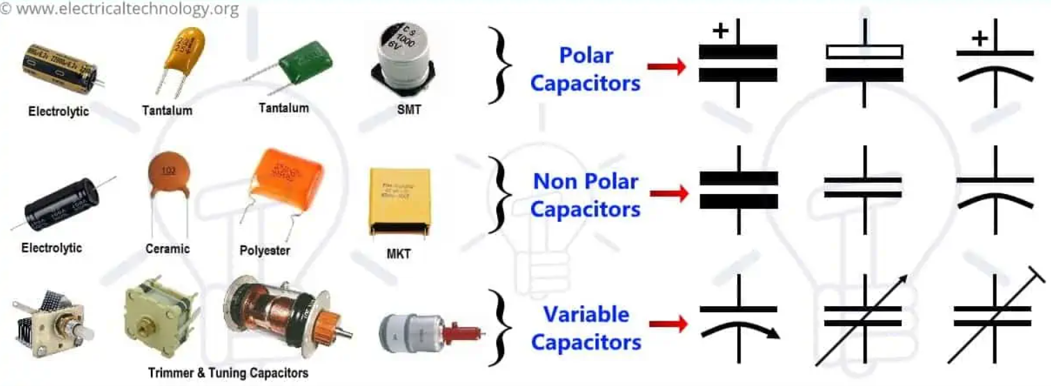
Capacitors are in different shapes and sizes. The picture below is showing the different types of capacitors and their symbol in circuit.
Now let’s consider a parallel-plate capacitor like a picture below:
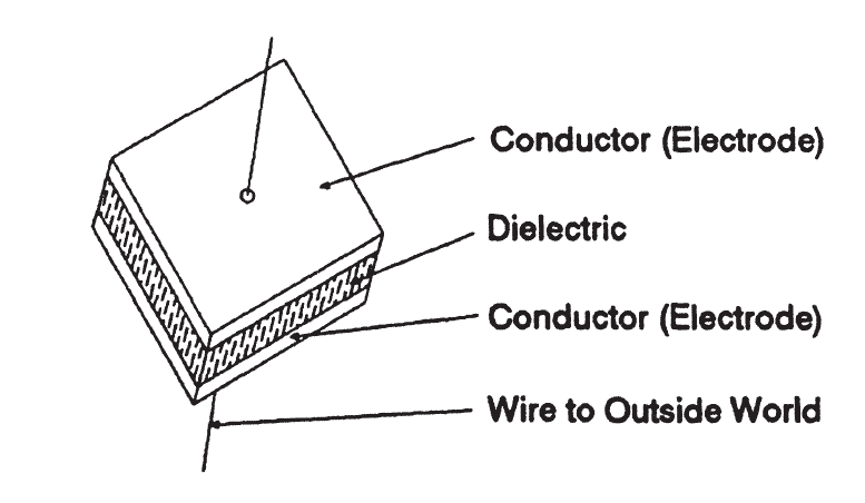
As you see, two conductors or electrodes separated by a dielectric material of uniform thickness. The conductors can be any material that will conduct electricity easily. The dielectric must be a poor conductor-an insulator.
1-2 Capacitors:Passive or Active?#
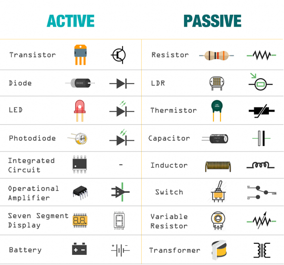
Capacitors are classified as passive elements in electrical circuits.
Passive elements do not provide power gain; they can store or dissipate energy but cannot generate it but active elements can provide power gain and can generate energy.In the picture below you can see examples of passive and active components:
1-3 Capacitor Applications:#
Energy Storage:
Capacitors are used to accumulate and discharge energy over varying periods.
They help smooth out pulsating direct current in filter circuits.
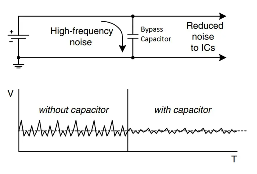
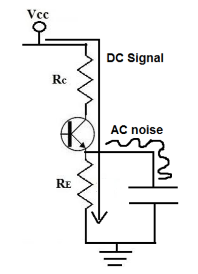
Bypass Capacitors:
A bypass capacitor, also known as a decoupling capacitor, is a capacitor used in electronic circuits to filter out unwanted noise from the power supply. It is typically placed between the power supply (VCC) and ground (GND) pins of an integrated circuit (IC). The bypass capacitor helps to smooth out voltage spikes and reduce power supply noise, ensuring that the circuit receives a clean and stable DC voltage.
These capacitors prevent the flow of direct current while allowing alternating current to pass.
They attenuate low-frequency currents while permitting higher frequencies to pass.
For further information you can visit these websites:
Reducing Radio Interference:
In combination with resistors, capacitors reduce radio interference caused by arcing contacts.
They also increase the operational life of the contacts.
For further information you can visit this website :
1-4 Capacitance derivation in flat capacitor:#
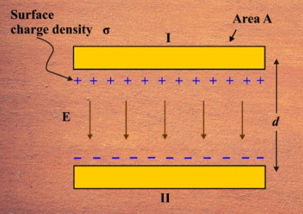
The capacitance ( C ) of a capacitor is defined as the charge ( Q ) stored per unit voltage ( V ) across its plates:
For a parallel plate capacitor, the electric field ( E ) between the plates is given by:
where:
( V ) is the voltage across the plates,
( d ) is the separation between the plates.
The electric field ( E ) is also related to the surface charge density ( \(\sigma\) ) on the plates(according to Gauss’s law.visit: https://phys.libretexts.org/Bookshelves/University_Physics/University_Physics_(OpenStax)/University_Physics_II_-Thermodynamics_Electricity_and_Magnetism(OpenStax)/06%3A_Gauss’s_Law/6.04%3A_Applying_Gausss_Law#:~:text=According%20to%20Gauss’s%20law%2C%20the,spherical%20surface%20of%20radius%20r.)
where:
\(( \epsilon_0 )\) is the permittivity of free space.
The surface charge density ( \(\sigma\) ) can be expressed as the charge ( Q ) per unit area ( A ):
Now we can substitute the expression for ( \(\sigma\) ) into the equation for ( E ):
From ( \(E = \frac{V}{d} \)):
\[ E = \frac{Q}{\epsilon_0 A} \]Setting these equal gives:
\[ \frac{V}{d} = \frac{Q}{\epsilon_0 A} \]Rearranging this equation to find ( Q ): $\( Q = \frac{\epsilon_0 A V}{d} \)$
Now, substitute ( Q ) back into the capacitance formula:
Thus, we arrive at the formula for the capacitance of a parallel plate capacitor:
If a dielectric material is present between the plates, the formula becomes:
where:
(C) is the capacity of parallel-plat capacitor
( \(\kappa\) ) is the relative permittivity of the dielectric material.
\(( \epsilon_0 )\) is the permittivity of free space.
(A) is the area of the plat.
(d) is the distance between two electrodes.
Now to get an idea of what a farad is, calculate the area which would be necessary in a capacitor built to have one farad, to operate in a vacum, and to have a spacing between electrodes of one millimeter.
That is why one farad capacitors aren’t made very often and when they are, they are never made with a vacuum dielectric and a one millimeter spacing.Note a tendency toward the higher values of \(\kappa\) for reasons that are now obvious. (With a \(\kappa\) of 10,that one farad capacitor area can be reduced to a 11.3 million square meters!)
The table below is showing the \(\kappa\) value for various materials :
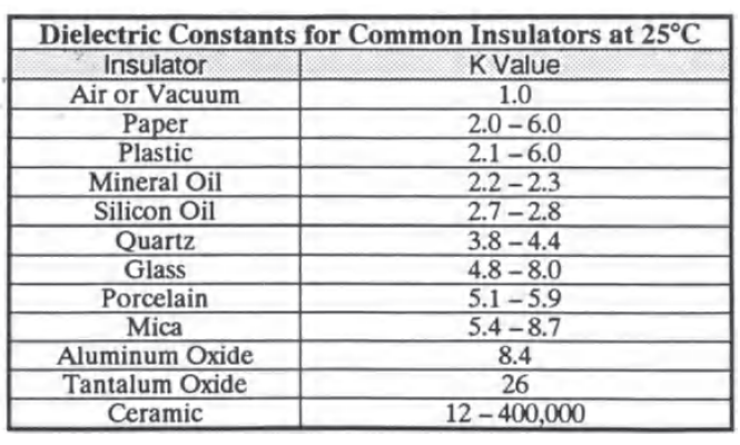
Capacitors used for commercial purposes are made from metallic foil interweaved with thin sheets of either Mylar or paraffin-impregnated paper. Small capacitors are typically made from ceramic materials and then sealed with epoxy resin.A typical question is why industry makes commercial capacitors with any-of the materials having low values of \(\kappa\). The answer generally lies with other capacitor characteristics such as stability with respect to temperature, voltage ratings, etc.
2- Capacitor behavior in a circuit:#
Consider the below circuit:
import schemdraw
from schemdraw import elements as elm

with schemdraw.Drawing() as d :
    elm.Switch().label('Switch')
    elm.Resistor().label('R')
    elm.Capacitor().down().label('C')
    elm.Line().length(d.unit*2).left()
    elm.Battery().up().label('battery','bot')

2-1 Charge curve:#
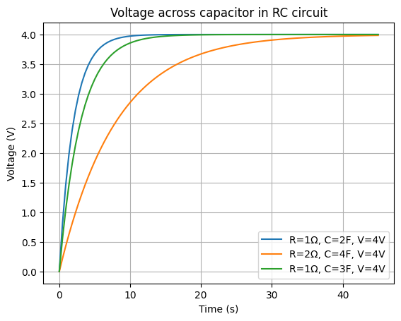
When the switch is closed, current from the battery flows through the circuit, charging the capacitor. When the capacitor is completely charged, no further current flows. At that time, the voltage across the capacitor would be equal to the supply voltage of the battery. Voltage across the capacitor advances from zero (fully discharged) to the supply voltage along some predetermined path with respect to time. If the resistor is small, current flows easily and the capacitor is charged more quickly. If the resistor is very large, the charging process follows a different path and will take longer to complete.The behavior of voltage versus time is also influenced by the size of the capacitor. If the capacitor’s capacitance is very large, it will require more total energy to fill, and current flowing through the resistor will require a longer time to charge it.
If we call the potential applied by the function generator during the positive half cycle V, then \( V = V_R + V_C = iR + \frac{q}{C} \). The current, i, is \( \frac {dq}{dt} \), and we have \( V = \frac {dq}{dt}\times R + \frac{q}{C} \). The solution to this differential equation is \( q = C\times V\times (1 - e^{-\frac{t}{RC})} \). Since the voltage across the capacitor is \(\frac{q}{C}\), we can also write this as \( V_C = V\times (1 - e^{-\frac{t}{RC}})\), which gives us the voltage across the capacitor as a function of time.Diagram below illustrates three charging curves, each approaching the same end point but along different paths.
import matplotlib.pyplot as plt
import numpy as np

# Define the constants
R1 = 1 # ohms
C1 = 2 # Farads
V1 = 4 # volts

R2 = 2 # ohms
C2 = 4 # Farads
V2 = 4 # volts

R3 = 1 # ohms
C3 = 3 # Farads
V3 = 4 # volts

# Define the time range
t = np.linspace(0, 45, 100) # Time from 0 to 45 seconds with 100 points

# Calculate V_C for each set of parameters
V_C1 = V1 * (1 - np.exp(-t / (R1 * C1)))
V_C2 = V2 * (1 - np.exp(-t / (R2 * C2)))
V_C3 = V3 * (1 - np.exp(-t / (R3 * C3)))


# Plot the graphs
plt.plot(t, V_C1, label=f'R={R1}Ω, C={C1}F, V={V1}V')
plt.plot(t, V_C2, label=f'R={R2}Ω, C={C2}F, V={V2}V')
plt.plot(t, V_C3, label=f'R={R3}Ω, C={C3}F, V={V3}V')

plt.xlabel('Time (s)')
plt.ylabel('Voltage (V)')
plt.title('Voltage across capacitor in RC circuit')
plt.grid(True)
plt.legend() # Add the legend to differentiate the plots
plt.show()
2-2 Characteristic time :#
The characteristic time of a capacitor in an RC (resistor-capacitor) circuit is known as the RC time constant, denoted by the Greek letter τ (tau). It is calculated as the product of the resistance (R) and the capacitance (C):
This time constant represents the time required for the voltage across the capacitor to either charge up to approximately 63.2% of its final value or discharge to about 36.8% of its initial value when a voltage is applied or removed.
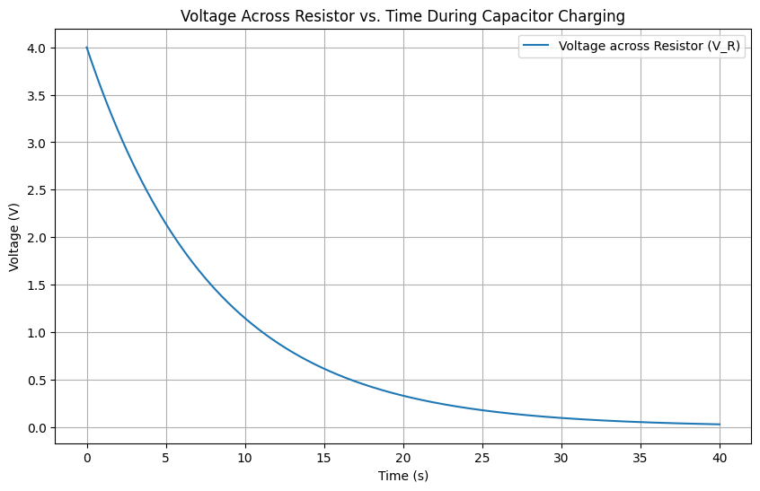
2-3 Resistor voltage during capacitor charging:#
We know that \( V = V_R + V_C = iR + \frac{q}{C} \) in this RC circuit. now that we find \(V_C\) we can easily obtain \(V_R\) which is voltage across resistor: \( V_R = V\times e^{-\frac{t}{RC}}\)
In the plot below you can see the voltage across resistor while capacitor is charging for orange curve (R = 2 Ohms and C = 4 F and V = 4 v) :
Note : The reason why the time axis is considered as 5 to the characteristic time is that the duration of charging the capacitor is approximately this value.
import numpy as np
import matplotlib.pyplot as plt

# Parameters
V = 4  # initial voltage in volts
R = 2  # resistance in ohms
C = 4  # capacitance in farads
tau = R * C  # time constant

# Time array
t = np.linspace(0, 5 * tau, 1000)  # 5 times the time constant

# Voltage across the resistor
Vr = V * np.exp(-t / tau)

# Plotting
plt.figure(figsize=(10, 6))
plt.plot(t, Vr, label='Voltage across Resistor (V_R)')
plt.xlabel('Time (s)')
plt.ylabel('Voltage (V)')
plt.title('Voltage Across Resistor vs. Time During Capacitor Charging')
plt.grid(True)
plt.legend()
plt.show()
2-4 How does an RC circuit work?#
Instantaneous Switch Closure: When the switch is first closed, the entire voltage of the battery appears across the resistor, and none across the capacitor. This is because initially, the capacitor acts like a short circuit for an instant.
Voltage Change Over Time: As time progresses, the voltage across the resistor decreases while the voltage across the capacitor increases. This change follows an exponential curve as the capacitor charges.
The RC circuit can be tailored to automate tasks based on how the voltage changes over time, which is incredibly useful in many practical scenarios, including automatic lighting systems.The circuit can be designed to operate a switch when the voltage across the capacitor reaches a certain level.If your application requires the switch to operate based on decreasing voltage (instead of increasing), you could use the voltage across the resistor, as shown in the plot above.
To find out more about automatic lighting system visit : https://en.wikipedia.org/wiki/Lighting_control_system
Once the capacitor in an RC circuit is fully charged, the behavior of the circuit changes significantly:
Capacitor Voltage Stabilizes: The voltage across the capacitor reaches the supply voltage (V0). At this point, the capacitor behaves like an open circuit.
Current Drops to Zero: As the capacitor charges, the current in the circuit decreases exponentially. Once fully charged, the current through the circuit becomes practically zero because the capacitor no longer allows any additional charge to flow.
Voltage Across Resistor is Zero: Since the current is zero, the voltage drop across the resistor also becomes zero (Ohm’s law: V = IR, where I is zero).
What Happens Next?
In a real-world application, what happens next depends on the circuit’s design:
Steady State: If the circuit is left as is, it will remain in a steady state with the capacitor holding the charge and no current flowing through the resistor.
Discharge Path: If the circuit includes a path for discharging the capacitor (like a switch), opening that path will allow the capacitor to discharge, causing the voltage across it to drop and current to flow again through the resistor.You can see the example of this situation in the section below :
import schemdraw
import schemdraw.elements as elm

with schemdraw.Drawing() as d:
    elm.Switch().label('switch1')
    d.push()
    elm.Resistor().label('R')
    elm.Capacitor().down().label('C','bot')
    elm.Line().left()
    d.pop()
    elm.Switch().down().label('switch2','bot')
    elm.Line().left()
    elm.Battery().up().label('battery')

2-5 Capacitor as storage battery:#
In the circuit above, When the switch 1 is closed, all the voltage of the battery is initially across the resistor. Over time, this voltage decreases as the capacitor charges up. This timing circuit is a typical DC application, emphasizing that once the capacitor is fully charged, it blocks the flow of DC current.
If switch 2 is closed to discharge the capacitor, the stored energy would flow through the resistor until the voltage across the capacitor drops to zero. The capacitor here acts similarly to a storage battery, holding charge and releasing it as needed, although the underlying principles are different.
3 Capacitor as filter:#
The storage capability of the capacitor is used to good effect in filters.
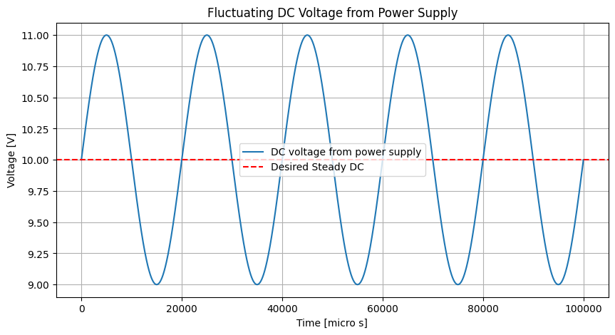
3-1 DC Analysis:#
A typical DC power supply offers a good case for an example. Basic DC power supplies provide an output (that is, the voltage across a load, shown in the circuit below as a resistor) which is fluctuating.
3-1-1 Circuit without capacitor:
The plot below is showing a situation where the voltage is flactuating.What is really wanted is a straight line(shown with red line in above figure) across this graph representing a steady DC voltage.
import schemdraw
import schemdraw.elements as elm

with schemdraw.Drawing() as d:
    elm.Source().up().label('power supply',rotate=True,fontsize=9)
    elm.Line().right()
    d.push()
    elm.Resistor().label('Load',fontsize=9).down()
    elm.Line().left()
    d.pop()
    elm.Line().down(d.unit*0.1)
    elm.Line().right()
    elm.MeterV().down(d.unit*0.8)
    elm.Line().left()

import matplotlib.pyplot as plt
from PySpice.Spice.Netlist import Circuit
from PySpice.Unit import *

# Create a circuit
circuit = Circuit('Fluctuating DC Voltage')

# Define the power supply with a fluctuating DC voltage
# Using a DC source with an AC component (sine wave)
circuit.SinusoidalVoltageSource(1, 'n1', circuit.gnd, amplitude=1@u_V, frequency=50@u_Hz, offset=10@u_V)

# Define a load resistor
circuit.R(1, 'n1', circuit.gnd, 1@u_kΩ)

# Simulate the circuit
simulator = circuit.simulator(temperature=25, nominal_temperature=25)
analysis = simulator.transient(step_time=1@u_us, end_time=100@u_ms)

# Plot the results
figure, ax = plt.subplots(figsize=(10, 5))
ax.plot(analysis['n1'])
plt.title('Fluctuating DC Voltage from Power Supply')
plt.xlabel('Time [micro s]')
plt.ylabel('Voltage [V]')
plt.grid()

# Add a horizontal line for average power
plt.axhline(y=10, color='r', linestyle='--')

plt.legend(['DC voltage from power supply', 'Desired Steady DC'])
plt.show()
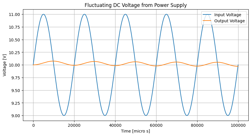
3-1-2 Circuit with capacitor:
To approach the desired straight line, add a capacitor to the circuit to smooth these fluctuations.
As you see in the plot below, capacitor is helping us to approach the desired straight line.In this plot, input voltage is the power supply voltage which is defined by the sinusoidal voltage source with the following properties:
DC offset: 10V
AC amplitude: 1V
Frequency: 50 Hz
So, the input voltage fluctuates around 10V, varying between 9V and 11V.So that we have a flactuating voltage source with this formula : \(V(t) = 10 + 1\times sin(2\pi \times 50t)\)
With the voltage at zero and the capacitor discharged, turn the supply on. As the voltage begins to rise, some current will flow to charge the capacitor while the rest passes through the resistor. Some time before the capacitor is completely charged, the voltage from the supply will begin to decline. As soon as the supply voltage is below the capacitor voltage, the capacitor will begin to discharge, and current will flow from the capacitor, tending to maintain the voltage across the resistor. If the value of capacitance is chosen correctly, the capacitor cannot be totally discharged during the time available, and the capacitor will be charged once more as the supply voltage exceeds the capacitor voltage.
import schemdraw
import schemdraw.elements as elm

with schemdraw.Drawing() as d:
    elm.Source().up().label('power supply',rotate=True,fontsize=9)
    elm.Line().right()
    d.push()
    elm.Capacitor().label('C').down()
    elm.Line().left()
    d.pop()
    elm.Line().right()
    elm.Resistor().label('Load',fontsize=10).down()
    elm.Line().left()

import matplotlib.pyplot as plt
from PySpice.Spice.Netlist import Circuit
from PySpice.Unit import *

# Create a circuit
circuit = Circuit('Fluctuating DC Voltage')

# Define the power supply with a fluctuating DC voltage
# Using a DC source with an AC component (sine wave)
circuit.SinusoidalVoltageSource(1, 'n1', circuit.gnd, amplitude=1@u_V, frequency=50@u_Hz, offset=10@u_V)

# Define a load resistor
circuit.R(1, 'n1', 'n2', 1@u_kΩ)

# Define a capacitor to smooth out the fluctuations (optional)
circuit.C(1, 'n2', circuit.gnd, 80@u_uF)

# Simulate the circuit
simulator = circuit.simulator(temperature=25, nominal_temperature=25)
analysis = simulator.transient(step_time=1@u_us, end_time=100@u_ms)

# Plot the results
figure, ax = plt.subplots(figsize=(10, 5))
ax.plot(analysis['n1'])
ax.plot(analysis['n2'])
plt.title('Fluctuating DC Voltage from Power Supply')
plt.xlabel('Time [micro s]')
plt.ylabel('Voltage [V]')
plt.grid()
plt.legend(['Input Voltage', 'Output Voltage'])
plt.show()
3-2 AC Analysis#
When a capacitor is subjected to alternating current, to the capacitor, it looks just like DC which is flowing in and flowing out again. The capacitor is alternately being charged, discharged, and then recharged in the opposite direction before being discharged again. One important fact to note is that the capacitor can never block the flow of AC but instead permits a steady flow of current.
import schemdraw
import schemdraw.elements as elm

with schemdraw.Drawing() as d:
    elm.SourceSin().up().label('AC generator')
    elm.Resistor().right().label('R')
    elm.Capacitor().down().label('C')
    elm.Line().left()

import matplotlib.pyplot as plt
from PySpice.Spice.Netlist import Circuit
from PySpice.Unit import *
import numpy as np

# Define different capacitance values
capacitance_values = [1@u_uF, 10@u_uF, 100@u_uF]  # 1µF, 10µF, 100µF

# Define colors for the lines
colors = ['#1f77b4', '#ff7f0e', '#2ca02c', '#d62728']  # Blue, Orange, Green, Red

plt.figure(figsize=(10, 6))

# Initialize a flag to control input voltage labeling
first_iteration = True

for i, C_value in enumerate(capacitance_values):
    # Define the circuit
    circuit = Circuit('RC Circuit')
    circuit.SinusoidalVoltageSource('input', 'input', circuit.gnd, amplitude=1@u_V, frequency=50@u_Hz)
    circuit.R(1, 'input', 'output', 1@u_kΩ)
    circuit.C(1, 'output', circuit.gnd, C_value)

    # Create a simulator
    simulator = circuit.simulator(temperature=25, nominal_temperature=25)

    # Run the transient simulation
    analysis = simulator.transient(step_time=1@u_us, end_time=100@u_ms)

    # Extract the time, input voltage, and voltage across the capacitor
    time = np.array([float(t) for t in analysis.time])
    v_input = np.array([float(analysis['input'][i]) for i in range(len(analysis.time))])
    v_c = np.array([float(analysis['output'][i]) for i in range(len(analysis.time))])

    # Plot the input voltage only once
    if first_iteration:
        plt.plot(time, v_input, linestyle='--', color=colors[3], label='Input Voltage', alpha=0.5)
        first_iteration = False
    else:
        plt.plot(time, v_input, linestyle='--', color=colors[3], alpha=0.5)

    # Plot the voltage across the capacitor
    plt.plot(time, v_c, color=colors[i], label=f'C = {C_value}')

plt.xlabel('Time [s]')
plt.ylabel('Voltage [V]')
plt.title('Voltage Across Capacitor vs. Time for Different Capacitors')
plt.grid(True)
plt.legend()
plt.show()
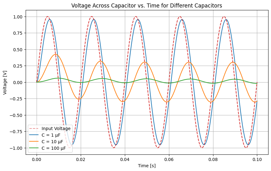
3-2-1 Analysis for different capacitances#
In the code above, we consider a sinusoidal voltage source which is : \(V(t) = V_a sin(2\pi f)\) . \(V_a\) is the amplitude of voltage which is 1V and f is considered 50 Hz and a resistor of 1kΩ and a capacitor are connected in series.An analysis is performed with a step time of 1 microsecond and an end time of 100 milliseconds. As you see, the voltage across the capacitor also has a sinusoidal curve.
Small Capacitance (1 µF):
The capacitor charges and discharges quickly.
The voltage waveform closely follows the input sinusoidal voltage.
Medium Capacitance (10 µF):
The charging and discharging rates are moderate.
The capacitor smooths out some of the fluctuations, but the voltage waveform still shows significant variations.
Large Capacitance (100 µF):
The capacitor charges and discharges slowly.
The voltage across the capacitor is much smoother and less responsive to rapid changes in the input voltage.
This behavior is consistent with the fact that larger capacitance values provide better filtering and energy storage but respond more slowly to changes in the input voltage.
Note: As you see, these plots are not completely sinusoidal but in bigger capacitace, it is more obvious.The reason is that a capacitor in an RC circuit will not pass high-frequency components well, and depending on the time constant (𝜏=𝑅⋅𝐶), it may smooth out the sinusoidal input voltage. This is especially true for larger capacitance values like 100 µF. The output voltage across the capacitor might be a smoother version of the input signal rather than a perfect sine wave.
import matplotlib.pyplot as plt
from PySpice.Spice.Netlist import Circuit
from PySpice.Unit import *
import numpy as np

# Define the frequencies to simulate
frequencies = [10@u_Hz, 50@u_Hz, 100@u_Hz]

for freq in frequencies:
    # Define the circuit
    circuit = Circuit('RC Circuit')
    circuit.SinusoidalVoltageSource('input', 'input', circuit.gnd, amplitude=1@u_V, frequency=freq)
    circuit.R(1, 'input', 'output', 1@u_kΩ)
    circuit.C(1, 'output', circuit.gnd, 10@u_uF)

    # Create a simulator
    simulator = circuit.simulator(temperature=25, nominal_temperature=25)

    # Run the transient simulation
    analysis = simulator.transient(step_time=1@u_us, end_time=100@u_ms)

    # Extract the time, input voltage, and voltage across the capacitor
    time = np.array([float(t) for t in analysis.time])
    v_input = np.array([float(analysis['input'][i]) for i in range(len(analysis.time))])
    v_output = np.array([float(analysis['output'][i]) for i in range(len(analysis.time))])

    # Plot the input and output voltage in one chart for each frequency
    plt.figure(figsize=(10, 6))
    plt.plot(time, v_input, label=f'Input Voltage @ {freq}')
    plt.plot(time, v_output, label=f'Capacitor Voltage @ {freq}')
    plt.xlabel('Time [s]')
    plt.ylabel('Voltage [V]')
    plt.title(f'Input and Capacitor Voltage vs. Time @ {freq}')
    plt.grid(True)
    plt.legend()
    plt.show()
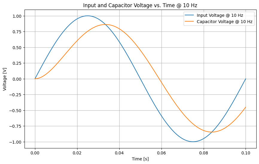
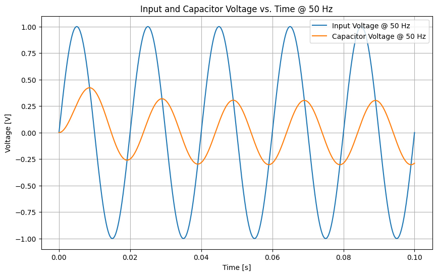
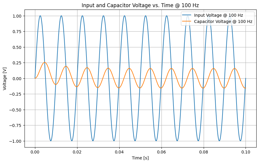
3-2-2 Analysis for different frequencies#
In this part, we use a sinusoidal voltage source, 1 k ohm resistor and 1 micro Farad capacitr. The plot above is showing the voltage across the capacitor for different frequencies.
Low Frequency (e.g., 10 Hz):
The capacitor has more time to charge and discharge within each cycle.
The voltage across the capacitor closely follows the input sinusoidal voltage.
Medium Frequency (e.g., 50 Hz):
The capacitor has less time to charge and discharge within each cycle compared to the low frequency.
The voltage across the capacitor still shows a sinusoidal pattern but with some delay and attenuation.
High Frequency (e.g., 100 Hz):
The capacitor has even less time to charge and discharge within each cycle.
The voltage across the capacitor is more attenuated and smooth compared to the input voltage. The capacitor acts as a low-pass filter, reducing the amplitude of the high-frequency components.
As the frequency increases, the capacitor’s voltage response becomes more attenuated and less responsive to rapid changes in the input voltage. This behavior is expected, as capacitors tend to filter out higher frequencies and smooth the voltage variations.
4- Reactance#
The capacitor, in an AC circuit, is acting something like a resistor in a DC circuit with the additional dimension of frequency to take into consideration.The two effects of frequency and capacitance are combined in an expression known as capacitive reactance and is expressed as \(X_C\).
Reactance is a concept in electrical engineering that describes how a circuit element opposes the flow of alternating current (AC) due to its inductance or capacitance. Unlike resistance, which affects both AC and DC, reactance specifically deals with AC and varies with the frequency of the signal.
Note that \(X_C\) is express in ohms, which is the unit of resistance.Reactance acts something like resistance, and uses the same unit in order to combine the two later.
The formula for determining \(X_C\) can be expressed as follows:
$\(
X_C = \frac{1}{2\pi f C}
\)$
Where:
\(X_C\) = capacitive reactance, ohm
\(\pi\) = 3.14
f = frequency, Hertz (cycles per second)
C = capacitance, Farads
There is a comparable expression for inductance which yields inductive reactive reactance. The unit of inductance is the Henry. It follows that inductance in an AC circuit impedes the flow of the current just as a capacitor does. The difference is that \(X_L\) is directly proportional to both frequency and inductance. The larger the inductor and the higher the frequency, the greater is the reactance to current flow: just the opposite of the behavior of a capacitor’s Xc.
The formula for determining \(X_L\) can be expressed as follows:
$\(
X_L = 2\pi f L
\)$
Where:
\(X_L\) = inductive reactance, ohm
\(\pi\) = 3.14
f = frequency, Hertz (cycles per second)
L = inductance, Henries
In the picture below you can see all of them :
import schemdraw
import schemdraw.elements as elm

with schemdraw.Drawing() as d:
    elm.SourceSin().up().label('AC generator')
    elm.Resistor().right().label('R')
    elm.Capacitor().down().label('C')
    elm.Inductor().left().label('L')

5- Impedance#
In practical applications, capacitors inherently possess some amount of resistance and inductance. This is because it is not feasible to manufacture capacitors that are entirely free of these properties. Therefore, when using capacitors in circuits, one must consider the effects of both resistance and inductance along with capacitance.In other words, a real capacitor is not a perfect capacitor as idealized in theory. It has additional characteristics that can influence its behavior in a circuit:
Resistance (R): Known as Equivalent Series Resistance (ESR), it represents the resistive losses in the capacitor.
Inductance (L): Known as Equivalent Series Inductance (ESL), it represents the inductive effects due to the leads and internal structure.
These factors must be taken into account when designing circuits, especially at higher frequencies where inductive effects become more significant.
Practical capacitor is with all three passive component properties: resistance, inductance and capacitance, and all capacitors actually look something like this. Of course, if the capacitor is a good one, the amount of resistance and inductance is very small compared to the amount of capacitance. In an AC circuit, all three components act to decrease the flow of current. The sum effect of all three is termed “impedance”. Unlike resistance, which only pertains to direct current (DC) circuits, impedance comprises both resistance (R) and reactance (X), therefore defining a complicated number expressed in ohms (Ω).
In electrical engineering, impedance, shown by the symbol “Z”, is a complicated number that defines the resistance a circuit offers to alternating current (AC). The convention for computing impedance is:
$\(
Z = R + jX
\)$
Where:
Z is impedance (in ohms),
R is resistance (in ohms),
jX is the reactance (in ohms),
j is the imaginary unit ( \(\sqrt{-1}\)). It indicates the phase difference between voltage and current, due to inductive or capacitive components,
X can be positive for inductive reactance or negative for capacitive reactance.
Inductive reactance is considered positive because the voltage across an inductor leads the current by 90 degrees. In mathematical terms, this phase lead is represented with a positive imaginary unit (j).Capacitive reactance is negative because the voltage across a capacitor lags behind the current by 90 degrees. This phase lag is represented with a negative imaginary unit (-j).
To calculate impedance, follow these steps:
Determine Resistance (R): Measure the resistance of the circuit
Calculate Inductive Reactance (XL)
Calculate Capacitive Reactance (XC):
Combine the Components: Plug the values of R and X (where \(X = X_L - X_C\)) into the impedance formula: Z = R + jX
The output will provide you both impedance’s magnitude and phase angle.Finally we have : $\( Z = R + j(X_L - X_C) \)\( Therefore, the value of ampedance is obtained from this formula : \)\( Z = \sqrt{R^2 +(X_L - X_C)^2} \)$
In the picture below you can see the different types of impedance :
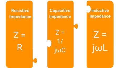
Capacitive Reactance(\(X_C\))decreases as frequency increases but inductive Reactance(\(X_L\))increases as frequency increases. Thus, in higher frequencies, capacitors act like inductors.
Self-Resonant Point: This is the frequency at which the capacitive reactance equals the inductive reactance.If there were no resistance in the circuit, the impedance would drop to zero at this point.
6- Concepts of Practical Capacitors:#
6-1 Impedance without resistance:#
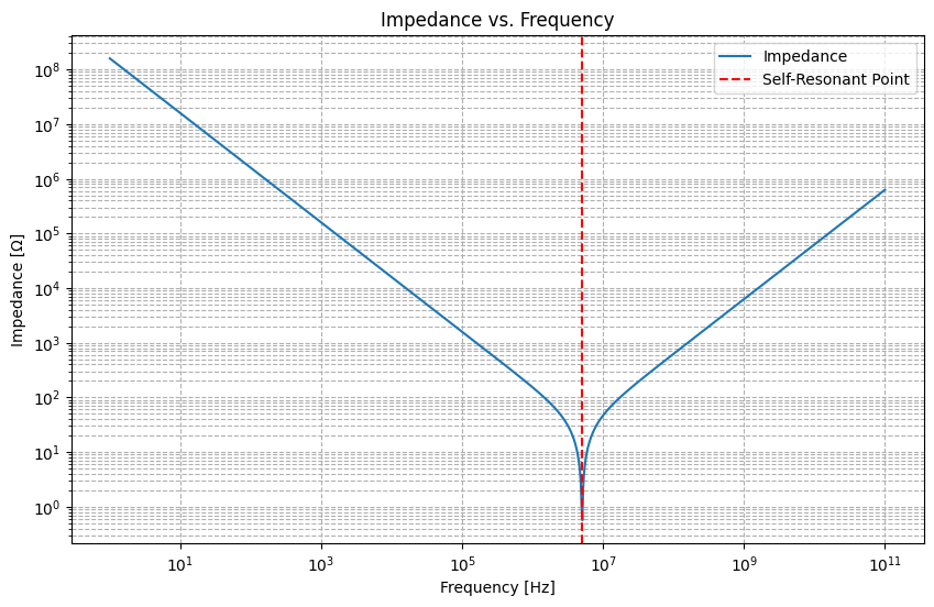
In the plot below, you can see the impedance vs. frequency in logarithmic scales when there is no resistance.In the left side of self-resonant point, reactance is capacitive and in the right side of self-resonant point, reactance is inductive .
note that the capacitance is considered as 1 nF and inductance is 1 µH and chart is for 10 Hz to 100 GHz frequency.The formula of impedance in this situation is : $\( Z = X_L - X_C = 2\pi f L - \frac{1}{2\pi f C} \)$
import matplotlib.pyplot as plt
import numpy as np

# Define the frequency range (logarithmic scale)
frequencies = np.logspace(0, 11, num=1000)  # from 1 Hz to 100 GHz

# Define constants for capacitance and inductance
C = 1e-9  # 1 nF
L = 1e-6  # 1 µH

# Calculate capacitive and inductive reactance
X_C = 1 / (2 * np.pi * frequencies * C)
X_L = 2 * np.pi * frequencies * L

# Calculate impedance
impedance = np.abs(X_C - X_L)

# Plotting
plt.figure(figsize=(10, 6))
plt.loglog(frequencies, impedance, label='Impedance')
plt.axvline(x=1 / (2 * np.pi * np.sqrt(L * C)), color='r', linestyle='--', label='Self-Resonant Point')
plt.xlabel('Frequency [Hz]')
plt.ylabel('Impedance [Ω]')
plt.title('Impedance vs. Frequency')
plt.grid(True, which="both", ls="--")
plt.legend()
plt.show()
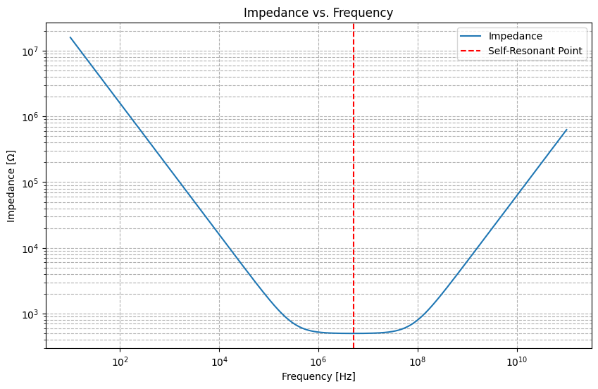
6-2 Impedance with resistance:#
Practical capacitors frequently look like plot below because they do include resistance. Exactly at the self-resonant point, in fact, they act entirely like a resistor.
note that the capacitance is considered as 1 nF and inductance is 1 µH and resistance is 500 ohms and chart is for 10 Hz to 100 GHz frequency.The formula of impedance in this situation is :
$\(
Z = \sqrt{R^2 +(X_L - X_C)^2} =\sqrt{R^2+(2\pi f L - \frac{1}{2\pi f C})^2}
\)$
import matplotlib.pyplot as plt
import numpy as np

# Define the frequency range (logarithmic scale)
frequencies = np.logspace(1, 11, num=500)  # from 10 Hz to 100 GHz

# Define constants for capacitance and inductance
C = 1e-9  # 1 nF
L = 1e-6  # 1 µH

# Calculate capacitive and inductive reactance
X_C = 1 / (2 * np.pi * frequencies * C)
X_L = 2 * np.pi * frequencies * L

# Calculate impedance
impedance = np.sqrt(500**2 + (X_L - X_C)**2)

# Plotting
plt.figure(figsize=(10, 6))
plt.loglog(frequencies, impedance, label='Impedance')
plt.axvline(x=1 / (2 * np.pi * np.sqrt(L * C)), color='r', linestyle='--', label='Self-Resonant Point')
plt.xlabel('Frequency [Hz]')
plt.ylabel('Impedance [Ω]')
plt.title('Impedance vs. Frequency')
plt.grid(True, which="both", ls="--")
plt.legend()
plt.show()
6-3 Ideal vs. Practical Capacitors:#
Ideal Capacitors: Would generate no heat when current flows.
Practical Capacitors: All practical capacitors have some resistance, known as Equivalent Series Resistance (ESR), and inductance. This resistance cannot be completely eliminated during manufacturing.When AC flows through a capacitor, the inherent resistance causes heat to build up. This limitation must be considered when designing circuits.
7- Practical Factors#
7-1 DF (Dissipation Factor):#
DF is a measure of the capacitor’s quality. It is the ratio of the capacitor’s resistance to its capacitive reactance. $\( DF = \frac {R}{X_C} = 2\pi fCR \)$ A higher DF indicates poorer performance. DF is often expressed as a percentage and is a preferred measurement over ESR (Equivalent Series Resistance) because it applies across a range of capacitance values without needing to specify capacitance.
ESR:
Pure resistance does not change with frequency. In practical capacitors, however, the simple series circuit does not exist, but rather there is a fairly complex mixture of resistance, capacitance and inductance. The result is that, as measured at the terminals of the capacitor, a resistance which declines with frequency. Because it really is not a pure resistance, it is called ESR or “Equivalent Series Resistance”. Manufacturers’ capacitor catalogs give graphs of ESR for many capacitors.
7-2 PF (Power Factor):#
The power factor is the ratio of the equivalent series resistance to the impedance of the device.The derivation of this factor is as follow : $\( PF = \frac {Power Losses}{Power In} \)\( \)\( PF = \frac{R\times I^2}{Z\times I^2} \)\( \)\( PF = \frac{R}{Z} \)$ Note:
“Power Factor” is used for capacitors when the PF is 10% or greater.
“Dissipation Factor” is used when the PF is less than 10%.
7-3 Corona Starting Voltage:#
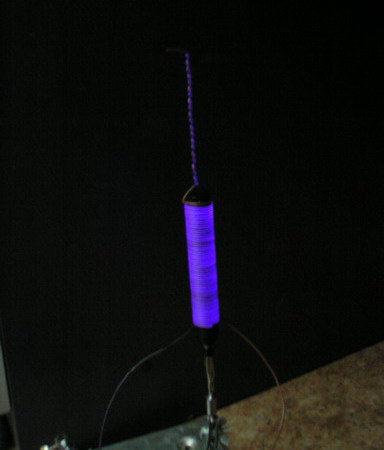
When capacitors operate above a certain voltage threshold, called the corona starting voltage, they can produce electrical noise and their lifespan may be reduced. Liquid-impregnated dielectrics generally have higher corona starting voltages compared to dry solid dielectrics.A corona discharge is an electrical discharge caused by the ionization of a fluid such as air surrounding a conductor carrying a high voltage.
In the picture below, you can see the corona discharge around a high-voltage coil:
7-4 Bias Voltage:#
All capacitors have a rated voltage that should not be exceeded by either DC voltage or peak AC voltage.
Film Capacitors and Ceramic Capacitors: These are non-polar devices, meaning they can operate with either positive or negative polarity.
Electrolytic Capacitors: These are polar devices and cannot tolerate much reverse voltage. Applying pure AC would result in the voltage being reversed half the time, which is not suitable for these capacitors.
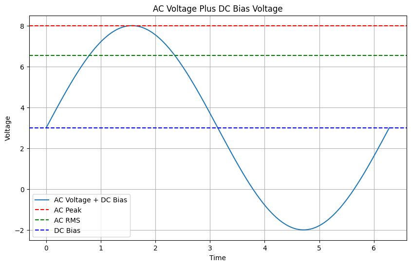
To address the issue with electrolytic capacitors, bias voltage is used. This involves applying both AC and DC voltage to the capacitor. The DC voltage is chosen to keep the AC voltage sufficiently above zero to prevent reversal, while also ensuring that the combined voltage does not exceed the rated voltage of the capacitor.
In the plot below, you can see the effect of bias voltage on a AC voltage.
import matplotlib.pyplot as plt
import numpy as np

# Time array
t = np.linspace(0, 2 * np.pi, 1000)

# AC voltage parameters
ac_peak = 5
ac_rms = ac_peak / np.sqrt(2)
dc_bias = 3

# AC voltage waveform
ac_voltage = ac_peak * np.sin(t)

# Total voltage with DC bias
total_voltage = ac_voltage + dc_bias

# Plotting the waveform
plt.figure(figsize=(10, 6))
plt.plot(t, total_voltage, label='AC Voltage + DC Bias')
plt.axhline(y=ac_peak + dc_bias, color='r', linestyle='--', label='AC Peak')
plt.axhline(y=ac_rms + dc_bias, color='g', linestyle='--', label='AC RMS')
plt.axhline(y=dc_bias, color='b', linestyle='--', label='DC Bias')


# Adding labels and title
plt.xlabel('Time')
plt.ylabel('Voltage')
plt.title('AC Voltage Plus DC Bias Voltage')
plt.legend()
plt.grid(True)
plt.show()
8- Trimmer Capacitor:#
A trimmer capacitor is a type of variable capacitor whose capacitance can be adjusted by manually changing the positioning of its conductive plates.Trimmer capacitors typically have two main applications: initial alignment and later restoration recalibration. When all fixed components are placed in a circuit, the resulting capacitance is often not precisely what was expected.Trimmer capacitors come in all shapes and sizes.
The image that follows is a PCB vertically mounted glass trimmer.
9- Effect of temperature on capacitor:#
Temperature can significantly impact the performance and characteristics of capacitors in several ways. Here are the key effects:
Capacitance Variation:
Polarized Dielectrics: The capacitance of capacitors with polarized dielectrics (like electrolytic capacitors) can change significantly with temperature. Generally, as the temperature increases, the capacitance increases.
Non-Polarized Dielectrics: Capacitors with non-polarized dielectrics (such as ceramic or film capacitors) tend to have more stable capacitance over a range of temperatures, but there can still be some variation.
Insulation Resistance:
As the temperature increases, the insulation resistance of a capacitor typically decreases. This is because higher temperatures can increase the conductivity of the dielectric material, leading to more leakage current.
Power Factor and Dissipation Factor:
Both the power factor and dissipation factor are affected by temperature. As the temperature rises, the dielectric losses increase, leading to a higher dissipation factor. This means more energy is lost as heat, reducing the efficiency of the capacitor.
For polarized dielectrics, higher temperatures can lead to significant increases in the power factor due to internal heating.
Voltage Handling Capability:
High temperatures can reduce a capacitor’s voltage handling capability. Exceeding the rated temperature can lead to breakdown of the dielectric material, potentially causing failure.
Life Span:
Terminal Seals and Joints: Changes in temperature can affect the mechanical structure of capacitors. Expansion and contraction of materials with different thermal coefficients can cause leaks at joints.
Frequency Response:
Temperature can also affect the frequency response of capacitors. At higher temperatures, the dielectric losses increase, which can affect the capacitor’s performance at higher frequencies.
Note : The term “dielectric losses” refers to energy lost in the form of heat within the dielectric material when an alternating current (AC) voltage is applied. This loss is mainly due to the internal friction within the dielectric as it polarizes and depolarizes with the changing AC voltage.
10- Reducing inductance by parallel connection:#
All capacitors have a small amount of inherent inductance due to their physical construction. This inductance can affect the performance of the capacitor, especially in high-frequency applications.By connecting a capacitor in parallel with a smaller capacitor (one with lower inductance), the overall inductance of the combination can be reduced. This is because the total inductance of two capacitors in parallel is less than the inductance of the smallest individual capacitor.Here is why : $\( \frac{1}{L_\text{total}} = \frac{1}{L_1}+\frac{1}{L_2} \)\( Therefore: \)\( L_\text{total} = L_1 \times \frac{L_2}{L_1+L_2} \)\( This means that the total inductance \)L_\text{total}\( will always be less than either of the individual inductances,\)L_1\( or \)L_2$.
11- Power Calculation:#
To calculate the power dissipated in a capacitor, you need to know the AC voltage across the capacitor and the AC current flowing through it.Although a DC (direct current) voltage can be present, a steady DC current cannot flow through a capacitor. This is because capacitors block steady DC after they are fully charged.However, if there’s a pulsating DC (a DC signal with an AC component), it must be treated as AC for the purpose of power calculation. The formula for power is : $\( 𝑃 = E I \)$ where :
𝑃 = Power in watts -
𝐸 = Potential (voltage) in volts
𝐼 = Current in amperes By using ohm’s law, (E=IR) : $\( P = R I^2 \)\( Ohm's Law for AC circuits may then be expressed as: \)\( E = I Z \)\( According to this form, power is calculated from the formula below : \)\( P = R \frac {E^2}{Z^2} \)$
12- AC Ripple:#
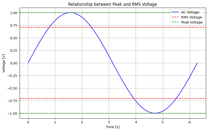
It refers to small, fluctuating AC components that can be superimposed on a DC signal, often seen in power supplies. These ripples are like minor waves on a pond, and capacitors help filter them out to produce a cleaner DC output. The expression for Ripple Voltage is as follows: $\( E = Z \sqrt{\frac{P}{R}} \)\( This AC voltage is known as the **"rms" voltage**.It is equal to the square root of two divided by two, or about 0.7 times the peak AC voltage. RMS stands for Root Mean Square, which is a way of expressing the effective or equivalent value of an alternating current (AC) voltage or current. It provides a measure of the AC signal that represents the same power dissipation as a corresponding direct current (DC) value.In AC circuits, the voltage and current are constantly changing, making it difficult to measure their true effect using simple averages. The RMS value helps quantify the power delivered by an AC signal as if it were a steady DC signal. For a sinusoidal voltage, the RMS value is calculated using the following formula: \)\( V_{\text{RMS}} = V_{\text{peak}} \times \frac{1}{\sqrt{2}} \)$ where:
\(V_{\text{RMS}}\): is the RMS voltage.
\(V_{\text{peak}}\): is the peak voltage of the AC signal.
Here is why :
In the plot below you can see the relation between rms voltage and AC voltage :
import matplotlib.pyplot as plt
import numpy as np

# Define the time range
t = np.linspace(0, 2 * np.pi, 1000)

# Sinusoidal waveform
voltage = np.sin(t)

# Calculate RMS value for a sinusoidal wave (peak value / sqrt(2))
rms_value = 1 / np.sqrt(2)

# Plotting the waveform
plt.figure(figsize=(10, 6))
plt.plot(t, voltage, label='AC Voltage', color='blue')
plt.axhline(y=rms_value, color='red', linestyle='--', label='RMS Voltage')
plt.axhline(y=-rms_value, color='red', linestyle='--')
plt.axhline(y=1, color='green', linestyle='--', label='Peak Voltage')
plt.axhline(y=-1, color='green', linestyle='--')

# Adding labels and title
plt.title('Relationship between Peak and RMS Voltage')
plt.xlabel('Time [s]')
plt.ylabel('Voltage [V]')
plt.legend()
plt.grid(True)

# Show plot
plt.show()
13- Conclusion:#
In this project, foundamentals of capacitors and its behavior are discussed. In section 1, types of capacitors and general applications of capacitors were presented along with theoretical relationships for their capacitance. In the second section, capacitor behavior in an RC circuit examined with PySpice. In section 3, the filtering capability of capacitors was discussed and examined in two modes: AC and DC.In the next two sections, impedance and reactance were explained.After that, these two parameters were explained with their practical application.Then, DF(Dissipation Factor), PF(Power Factor), Corona starting voltage, Bias Voltage, trimmer capacitors, effect of temperature on capacitor and Reducing inductance by parallel connection were explained.In the end, power calculation for capacitor and AC ripple were explained carefully and in the last section, all the sources except capacitor handbook, which is the main source, were cited.